Astrometric Corrections

Because we are combining the data from two different instruments, there are corrections that must be made to the coordinates of the X-ray sources such that it is propely in line with the coordinate system of HST. There will be some intrinsic amount of uncertainty in the XRBs’ coordinates due to the differences in the X-ray and optical resolution of their respective instruments. These are accounted for by defining 1- and 2-\(\sigma\) regions around each XRB, which trace out the regions within which we are 68% and 95% sure that the source falls. These regions are calculated using the information obtained through the astrometric correction process — namely, the standard deviation of the median offset between optical and X-ray coordinates. This Chapter outlines how to conduct an astrometric correction and calculate the 1- and 2-\(\sigma\) positional uncertainty regions around each XRB.

Calibrator Selection

To calibrate between X-ray and optical source coordinates, we need to select a sample of optical sources that we are reasonably certain are producing the X-ray emissions we detect. These include background galaxies (AGN and quasars), foreground stars, and isolated globular clusters (for example, Fig. 13). To find these sources, we must plot the coordinates of each X-ray source onto the HST image. We then identify the X-ray sources and their optical counterparts that are best suited for the assessment. You will want to pull the coordinates for each selected X-ray source, and (if you choose to do a by-hand correction) their associated optical source.

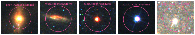
Fig. 13 Examples of X-ray sources that can be used as calibrators for the astrometric correction. The first 3 images are of AGN and quasars, based on their shapes and/or extremely red colors. The 4th is a foreground star, identifiable by the diffraction spikes. The last is a (somewhat) isolated globular cluster, based on the shape, color, and size relative to typical stars in M101.

Correction Calculation and Application

Astrometric corrections are handled by the function XRBID.Align.CorrectAstrometry(). It takes in the coordinates of your selected X-ray sources (cat_coords) and finds the nearest optical source from the coordinates of some base catalog (base_coords, which in this case are the coordinates from the DAOStarFinder catalog from Using AutoPhots.RunPhots() for Everything). Alternatively, you can calculate the astrometric correction yourself by hand-selecting the best optical source position of each calibrator and finding the median x- and y-coordinate offset between the optical and X-ray positions, as well as the standard deviation of those offsets.

If the standard deviations on the offsets are larger than the median offsets, then that suggests the CXO sources are already well-aligned with the HST image and no coordinate shift is necessary. The standard deviations on those shifts, however, are still needed to calculate the positional uncertainties, as it represents the variations in where the optical counterparts fall with respect to the X-ray coordinates of the selected sources. Ideally these will be small, but they’re expected to be non-zero.

Below is the code I use to find the X-ray calibrators and call CorrectAstrometry to calculate the correction:

import pandas as pd 
from XRBID.WriteScript import WriteReg
from XRBID.Sources import LoadSources, GetCoords
from XRBID.DataFrameMod import RemoveElse, FindUnique
from XRBID.Align import CorrectAstrometry

# Reading in sources from the DataFrame containing all of the X-ray sources
# You can use pd.read_csv() instead of LoadSources, if you prefer
M101_CSC = LoadSources("../testdata/cscresults_M101_renamed.frame")

# Find X-ray sources with a unique CSC ID,
# in case multiple rows in the the DataFrame have the same CSC ID
M101_unique = FindUnique(M101_CSC, header="CSC ID")

# Saving M101 to a region file that can be opened in DS9
WriteReg(M101_unique, outfile="../testdata/M101_cscsources.reg", idname="CSC ID", 
         radius=10, radunit="arcsec", width=2, color="hotpink", showlabel=True)

Reading in sources from ../testdata/cscresults_M101_renamed.frame...

Saving ../testdata/M101_cscsources.reg

The code above reads in the DataFrame (CSV) file containing the X-ray sources (created in Converting from VOTable to Pandas DataFrame) and saves a region file of these sources called M101_cscsources.reg. By default, because this DataFrame only contains RA and Dec for coordinates, WriteReg() will save a region file using galaxy coordinate units (fk5 in DS9). I define the color as hotpink (the default is a variation on yellow) and label each source with the CSC ID, as defined by idname and showlabel. You can pass any header in your DataFrame under idname, and it will use those entries to label each of the sources/regions.

Open whatever image you want to align these sources to in DS9 (I use the F555W mosaic file created in Creating Mosaics with AstroDrizzle) with Region > Open. Then, inspect the image to select a handful of good astrometric calibrator sources (see Fig. 13). Save the CSC ID names of these sources in a list, and pull the information for these sources from the DataFrame; the RemoveElse() function from XRBID.DataFrameMod is useful for removing all entries except for those that match the IDs in your list.

# List of source names to use as calibrators in the Astrometric Correction
# These I identified manually by inspecting the HST image in DS9 with the 
# regions saved above plotted over the image
M101_calibrators = ['2CXO J140251.0+542420', 
                    '2CXO J140248.0+542403', 
                    '2CXO J140356.0+542057',
                    '2CXO J140355.8+542058',
                    '2CXO J140357.6+541856',
                    '2CXO J140339.3+541827',
                    '2CXO J140346.1+541615',
                    '2CXO J140253.3+541855',
                    '2CXO J140252.1+541946']

print(len(M101_calibrators), "calibrators to match...")

# Using DataFrameMod.RemoveElse() to remove all but the sources above from the DataFrame
M101_calibrators = RemoveElse(M101_unique, keep=M101_calibrators, header="CSC ID")
print(len(M101_calibrators), "calibrators found.")

# Saving these as a region file, in case we want to double-check
WriteReg(M101_calibrators, outfile="../testdata/M101_calibrators.reg", radius=25, width=2)

9 calibrators to match...
9 calibrators found.
Saving ../testdata/M101_calibrators.reg

For CorrectAstrometry, the catalog coordinates you’ll want to use are the coordiates of the calibrators, while the base coordinates you’re aligning them to come from the source extraction conducted in Using AutoPhots.RunPhots() for Everything. Make sure you’re using the same coordinate system for both lists (in my case, I’m using the galaxy coordiates, which are designated fk5 in DS9. Thus, I pull the base coordinates from M101_daofind_f555w_acs_fk5.reg).

# Setting up the base and the catalog coordinates for CorrectAstrometry
base_coords = GetCoords("testdata/M101_daofind_f555w_acs_fk5.reg")
cat_coords = [M101_calibrators["RA"].values.tolist(), 
              M101_calibrators["Dec"].values.tolist()]

# Running CorrectAstrometry
CorrectAstrometry(base_coords, cat_coords, returnshifts=True, \
                  savebasereg="testdata/M101_astrocorrect.reg")

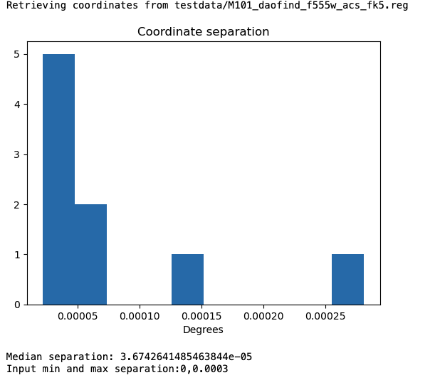
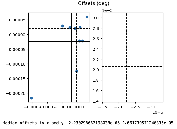
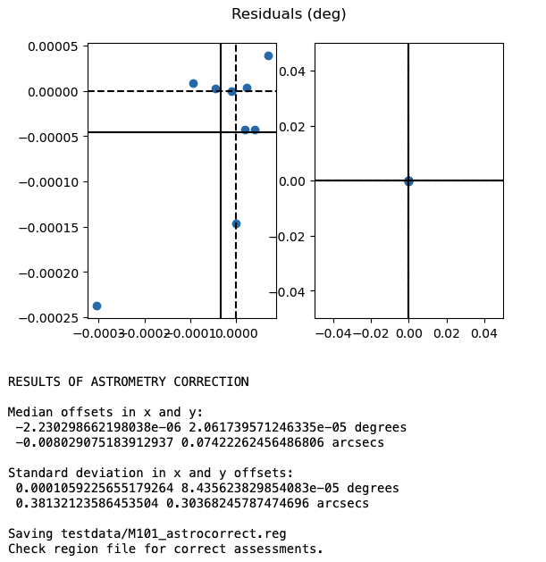
Here we see that the median x and y shifts are smaller than their standard deviation. This means the alignment is already pretty good and that we just need to use the standard deviations to calculate the positional uncertainty radii! Otherwise, you will want to take the median shifts and apply this astrometric correction to the coordinates of your X-ray catalog. CorrectAstrometry will not do this for you!

Calculating Positional Uncertainty

Because of different instrumental resolutions and inherent uncertainties, it isn’t possible to know the exact location of an X-ray source on the HST optical image, but the positional uncertainty defines a region within which we are reasonably certain the X-ray source falls. This is defined by 1- and 2-\(\sigma\) radii, representing the region within which the source has a 68% and 95% chance of being found.

There are two components that go in to the positional uncertainty estimation: the X-ray positional uncertainty, and the standard deviation on the astrometric correction above. The X-ray positional uncertainty is due to the fact that the PSF of CXO increasingly degrades for sources that are an increasing distance from the telescope’s main pointing at the time of the observation. That is, the farther the X-ray source is from the center of the image, the harder it is to tell where those detected X-rays came from.

The X-ray positional uncertainty is obtained using Equations 12 and 14 from [KKW+07]:

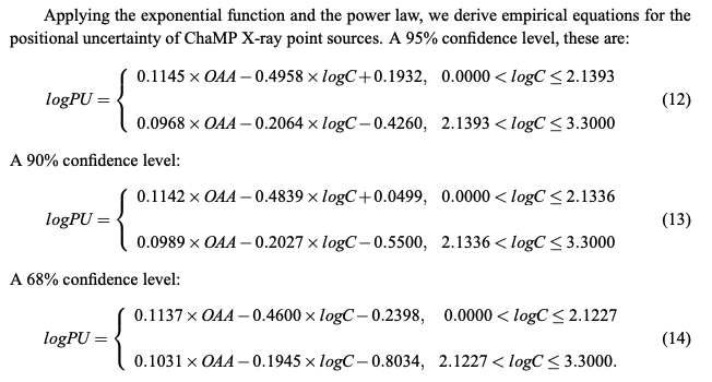
The source counts and the off-axis angle are src_cnts_aper_b and theta or theta_mean from Retrieving X-ray Data from the CSC, which I renamed Counts and Theta in my DataFrame.

The positional uncertainties from the standard deviations are added in quadrature to the X-ray uncertainties, meaning you sum the squares of the uncertainties and take the square root. So for 1- and 2-\(\sigma\), you’d combine the positional uncertainties from the equations above (let’s call them sig1_kim and sig2_kim) with those from the standard deviations on the astrometric correction (xstd and ystd) thus:

from numpy import sqrt

sig_astro = sqrt(xstd**2 + ystd**2)
sig1 = sqrt(sig1_kim**2 + sig_astro**2)
sig2 = sqrt(sig2_kim**2 + (2*sig_astro)**2) # 2sig is literally twice 1sig for the std-derived p.u.

All of these steps are handled by Align.CalcPU():

from XRBID.Align import  CalcPU

# Takes in DataFrame or Off-axis Angle/Counts and returns 1 and 2sig
# NOTE: theta needs to be in arcminutes, which is the default CSC unit
sig1, sig2 = CalcPU(M101_CSC, std=[0.3813,0.3037])

CalcPU calculates the total 1- and 2-\(\sigma\) positional uncertainty from both the X-ray data and the input standard deviations on the astrometric correction. This can be saved directly into to your DataFrame:

M101_CSC['1Sig'] = sig1  # Saves sig1 to a new header called '1Sig'
M101_CSC['2Sig'] = sig2  # Saves sig2 to a new header called '2Sig'

# The new DataFrame has 1 and 2sig added at the end of the columns list
display(M101_CSC)

M101_CSC.to_csv('../testdata/M101_csc_astrocorrected.frame')

	Separation	CSC ID	RA	Dec	ExpTime	Theta	Err Ellipse Major	Err Ellipse Minor	Err Ellipse Angle	Significance	...	HM Ratio lolim	HM Ratio hilim	MS Ratio	MS Ratio lolim	MS Ratio hilim	Counts	Counts lolim	Counts hilim	1Sig	2Sig
0	0.835778	2CXO J140312.5+542056	210.802227	54.348952	192658.710333	2.687974	0.296164	0.295254	89.606978	22.302136	...	-0.100562	0.156777	-0.553404	-0.61649	-0.485322	170.006026	155.698239	184.313814	0.499641	1.003207
1	0.835778	2CXO J140312.5+542056	210.802227	54.348952	142729.493705	2.727056	0.296164	0.295254	89.606978	22.302136	...	-0.100562	0.156777	-0.553404	-0.61649	-0.485322	254.489381	233.532285	274.136658	0.498084	0.999338
2	0.835778	2CXO J140312.5+542056	210.802227	54.348952	141298.623812	2.783596	0.296164	0.295254	89.606978	22.302136	...	-0.100562	0.156777	-0.553404	-0.61649	-0.485322	442.576953	419.112035	464.477543	0.496277	0.994895
3	0.835778	2CXO J140312.5+542056	210.802227	54.348952	132129.439441	2.690653	0.296164	0.295254	89.606978	22.302136	...	-0.100562	0.156777	-0.553404	-0.61649	-0.485322	131.798703	118.539780	144.321019	0.502819	1.014894
4	0.835778	2CXO J140312.5+542056	210.802227	54.348952	130186.649966	2.749161	0.296164	0.295254	89.606978	22.302136	...	-0.100562	0.156777	-0.553404	-0.61649	-0.485322	649.590529	616.129127	683.051932	0.494942	0.991738
...	...	...	...	...	...	...	...	...	...	...	...	...	...	...	...	...	...	...	...	...	...
3487	892.520732	2CXO J140447.2+542633	211.196627	54.442543	120993.038017	NaN	1.612100	0.795238	86.007749	2.650000	...	NaN	NaN	NaN	NaN	NaN	0.000000	0.000000	59.364933	0.487466	0.974933
3488	892.520732	2CXO J140447.2+542633	211.196627	54.442543	88598.047743	NaN	1.612100	0.795238	86.007749	2.650000	...	NaN	NaN	NaN	NaN	NaN	0.000000	0.000000	14.952548	0.487466	0.974933
3489	892.520732	2CXO J140447.2+542633	211.196627	54.442543	81021.851289	13.486809	1.612100	0.795238	86.007749	2.650000	...	NaN	NaN	NaN	NaN	NaN	53.481053	29.414579	77.547526	3.190131	7.658538
3490	892.520732	2CXO J140447.2+542633	211.196627	54.442543	52087.100775	NaN	1.612100	0.795238	86.007749	2.650000	...	NaN	NaN	NaN	NaN	NaN	0.000000	0.000000	34.780341	0.487466	0.974933
3491	892.520732	2CXO J140447.2+542633	211.196627	54.442543	14276.493764	3.416463	1.612100	0.795238	86.007749	2.650000	...	NaN	NaN	NaN	NaN	NaN	7.591890	4.313574	10.870206	0.738103	1.710737

3492 rows × 30 columns

Selecting the best 2-\(\sigma\) radius per source

Depending on what information you chose to pull from CSCview, you may see that some sources have multiple observations listed in your DataFrame. These different observations may have different 2-\(\sigma\) radii associated with them. To get the best localization of each X-ray source, we should select the observation with the smallest 2-\(\sigma\). I use the code below to select what I think is likely the best observation (though you may make arguments for using a different method, depending on the project):

from XRBID.DataFrameMod import BuildFrame, Find

# Pulling the ID of each unique CSC source
ids = FindUnique(M101_CSC, header="CSC ID")["CSC ID"].values.tolist()

# Building an empty DataFrame, which I will fill below
M101_best = BuildFrame()

for i in ids: # for each unique ID pulled from CSC...
    
    # Search for all instances (i.e. observations) of each source
    Temp = Find(M101_CSC, "CSC ID = " + i)
    
    # Try to avoid sources where counts = NaN (invalid observations) 
    if len(Find(Temp, ["Counts != NaN", "Theta != NaN"])) > 0: 
        Temp = Find(Temp, ["Counts != NaN", "Theta != NaN"])
    
    # Specifically focus on those with a valid number of counts
    if len(Find(Temp, "Counts > 0")) > 0: 
        Temp = Find(Temp, ["Counts > 0"])
        
    # Otherwise, all instances with counts = 0 have the same measurements, 
    # so it doesn't matter which row is chosen for the best radii
    else: pass;
    
    # Take the source with the smallest 2sig. 
    # If there's more than one, take the first on the list.
    Tempbest = Find(Temp, "2Sig =< " + str(min(Temp["2Sig"]))).iloc[:1]
    
    # Add the chosen source observation to the new DataFrame
    M101_best = pd.concat([M101_best, Tempbest], ignore_index=True)

# Saving results to a DataFrame file
# This file contains only rows from M101_CSC that has the 
# best 2sigma radius, based on the search performed above
M101_best.to_csv("../testdata/M101_csc_bestrads.frame")

display(M101_best)

	Separation	CSC ID	RA	Dec	ExpTime	Theta	Err Ellipse Major	Err Ellipse Minor	Err Ellipse Angle	Significance	...	HM Ratio lolim	HM Ratio hilim	MS Ratio	MS Ratio lolim	MS Ratio hilim	Counts	Counts lolim	Counts hilim	1Sig	2Sig
0	0.835778	2CXO J140312.5+542056	210.802227	54.348952	98379.672624	1.280763	0.296164	0.295254	89.606978	22.302136	...	-0.100562	0.156777	-0.553404	-0.616490	-0.485322	234.492581	216.678502	252.306660	0.493011	0.988256
1	1.951564	2CXO J140312.7+542055	210.803345	54.348663	49085.676020	4.725025	0.548072	0.380093	86.863933	2.648649	...	-0.080575	1.000000	-0.999375	-1.000000	-0.715178	209.970149	192.843759	227.096539	0.516471	1.038077
2	2.480949	2CXO J140312.5+542053	210.802221	54.348072	98379.672624	1.321652	0.296164	0.295733	84.016491	19.554042	...	0.026858	0.158026	-0.316052	-0.364147	-0.265459	252.846172	234.295673	271.396671	0.492957	0.988086
3	5.227586	2CXO J140313.1+542052	210.804553	54.347994	132129.439441	2.762119	0.880650	0.578584	29.467809	3.421053	...	0.130543	0.906309	-0.868207	-0.973766	-0.718926	23.229213	16.216620	30.241806	0.561749	1.188360
4	9.124404	2CXO J140313.5+542053	210.806667	54.348188	98379.672624	1.410741	0.633314	0.466131	58.539300	1.739130	...	0.194254	1.000000	-0.999375	-1.000000	-0.370394	7.040343	2.992146	11.088540	0.593981	1.300029
...	...	...	...	...	...	...	...	...	...	...	...	...	...	...	...	...	...	...	...	...	...
550	883.411465	2CXO J140138.8+541527	210.411860	54.257747	132129.439441	12.087047	8.647887	6.103176	111.468541	4.277778	...	-0.113054	0.935041	-0.792005	-0.932542	-0.617739	76.034629	52.273807	99.795450	1.921653	4.517698
551	884.529187	2CXO J140450.6+541721	211.211172	54.289330	139822.610581	9.951487	1.357801	1.057531	95.305118	8.976584	...	-0.099313	0.204247	-0.374766	-0.472829	-0.270456	155.562531	135.448493	174.718757	0.793067	1.558488
552	886.380054	2CXO J140216.3+543313	210.567813	54.553731	131222.705704	13.887674	2.480733	2.445301	115.654637	6.783292	...	-0.025609	0.271705	-0.222361	-0.322923	-0.118051	149.738677	121.454705	176.358886	1.676834	3.103807
553	890.405834	2CXO J140445.4+541452	211.189426	54.247897	139819.410649	10.703677	4.581313	2.651713	135.472019	4.411765	...	0.005621	0.434104	0.999375	0.501562	1.000000	NaN	NaN	NaN	0.487466	0.974933
554	892.520732	2CXO J140447.2+542633	211.196627	54.442543	14276.493764	3.416463	1.612100	0.795238	86.007749	2.650000	...	NaN	NaN	NaN	NaN	NaN	7.591890	4.313574	10.870206	0.738103	1.710737

555 rows × 30 columns

Saving the positional uncertainties as region files

You now have the RA and Dec of each source (ideally updated based on the results from your astrometric correction) and the best positional uncertainty radii of each one. Save these radii as region files that can be plotted over the HST image in DS9 using WriteScript.WriteReg():

# Saving the 1 and 2 sigma region files for DS9 use.
# The 2sig region files have the CSC ID printed above each source.
WriteReg(M101_best, radius=M101_best['2Sig'].values.tolist(), radunit='arcsec', \
         idname="CSC ID", showlabel=True, outfile='../testdata/M101_bestrads_2sig.reg')
WriteReg(M101_best, radius=M101_best['1Sig'].values.tolist(), radunit='arcsec', \
         outfile='../testdata/M101_bestrads_1sig.reg')

Saving ../testdata/M101_bestrads_2sig.reg
Saving ../testdata/M101_bestrads_1sig.reg

Now when you plot these region files on your HST image in DS9, you will see exactly where each XRB is expected to be found and which optical sources are associated with them. From here, we can get into the optical analysis, including: selecting the correct optical counterpart, extracting their photometric properties, and comparing those properties to theoretical models to estimate the donor star mass!

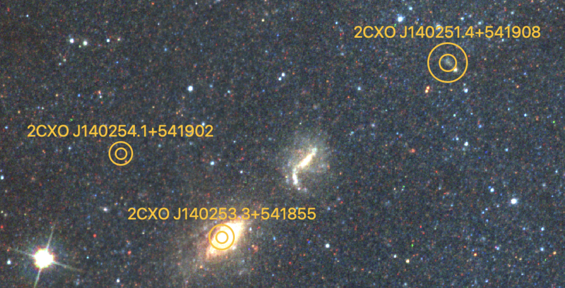
Fig. 14 Examples of the 1- and 2-\(\sigma\) positional uncertainties of CXO sources on an HST image, after applying the astrometric correction. By eye, the central source is clearly associated with a background galaxy, while the others are likely genuine XRBs.