HST Source Identification and Photometry

Photometry refers to measuring the amount of light that is emitted by a source (like a star, cluster, or galaxy) and detected by an instrument. The photometry is obtained by integrating the amount of flux detected within a given region (i.e. the aperture around the star), for a given filter (e.g. red, green, or blue). For our purposes, we convert this flux into a magnitude (I for red, V for green, B for blue) and can use these values to calculate the colors of each source (e.g. V-I, B-V, B-I), allowing us to conduct a deeper analysis of the source’s properties.

There are plenty of packages one can use to pull this data from an HST FITS file[1], but my preferred method is using the fleet of tools within the python package photutils. For my process, I set up a complete pipeline in the function PhotRun() in the AutoPhots.py script, but I’ll explain the steps for identifying HST point sources manually as well.

Note

While it is recommended to run AstroDrizzle through command line python, the scripts introduced here (and all others suggested in this guide) are fine to run within an iPython notebook. Just be sure to activate the proper environment (in my case, using conda activate stenv) before running jupyter notebook & in the command line. This will ensure your iPython notebook has access to all of the necessary python tools that were previously installed.

Using AutoPhots.RunPhots() for Everything

Assuming you don’t mind black boxes, the quickest way to extract and correct the photometric data from HST is to simply run my RunPhots() function. This code will take care of all photometric and aperture correction steps for you, with some input from the user. The basic steps it takes are:

• Find point sources with photutils.detection.DAOStarFinder;

• Measure the photometry within apertures with radius ranging from 1 to 30 pixels with photutils.aperture.CircularAperture;

• Calculate the apparent magnitudes of each object at each aperture radius;

• Calculate an aperture correction from 3–20 pixels (by default) and 20–infinity by prompting user to identify ‘ideal’ stars; these ideal stars are also used to calculate aperture corrections from 10–20 (by default) and 20–infinity pixels for extended sources (i.e. clusters);

• Apply aperture corrections to the apparent magnitudes and return the aperture correction factor and the correction error (both for point sources and extended sources as of version 1.5.0);

Running this code is fairly easy, but before you do, you will need to know the FWHM (full width at half maximum, the width of a Gaussian at half of its maximum height, as demonstrated in Fig. 8) of stars within the FITS file of interest. This can be measured within DS9[2]. Open your FITS file (be sure to set the scaling to something visible) and navigate to a relatively dark area with bright, isolated stars; you may have to set your cursor to pan using Edit > Pan first. Once in a good location, set your cursor to create a new region by selecting Edit > Region. Then under the Region menu located in the upper menu bar, go to Shape > Annulus. Click and drag somewhere on the image to create the annulus region. This region will be used to make a measurement of the radial profile of stars in this image, which will be used to estimate their FWHM.

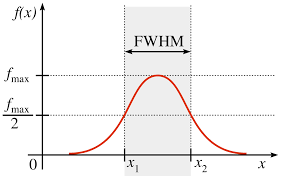
Fig. 8 Example of the FWHM of a Gaussian. Compare to Fig. 9, which plots only half of a Gaussian and, thus, gives the HWHM.

To take a good radial profile of a star, you will need to update this region to include more than a single annulus. Double-click on the region to open up the Annulus properties window. You can add additional annuli by changing the inner and outer radius and increasing the annuli count. For me, I chose inner and outer radii of 1 and 31 pixels, and plotted 20 annuli. Click Generate followed by Apply to update your annulus region. You can save this region for later use under Region > Save. I recommend saving it using image coordinates, so that you can reuse the same region on different galaxies.

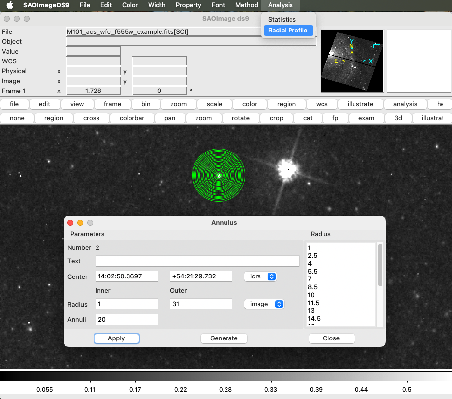
Fig. 9 Example of defining a region with several annuli, and the selection of Analysis > Radial Profile from the top menu.

To measure the radial profile of a star, click and drag your region to center it on a bright, isolated star. Select the Annulus window (or double-click to bring it back up) and select Analysis > Radial Profile from the top menu bar (shown in Fig. 9). This will open a new window with the radial profile of the star (Fig. 10). Estimate the FWHM by eye. Do this for a few stars to get a good idea of a reasonable estimate. You will use this value whether you’re using RunPhots or doing your own source identification with DAOStarFinder in the next section.

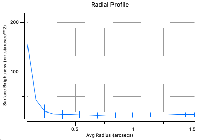
Fig. 10 Example radial profile of an HST star. In this case, half-max occurs at around 0.15 arcseconds, so the FWHM of this star would be 0.3 arcseconds. Beware: you’ll want to ensure you’re looking at stars and not clusters, which will have a much broader FWHM and likely a higher peak surface brightness.

You will also want to determine a good aperture radius with which to extract the photometry of compact star clusters, which will be read in to RunPhots() as extended_rad. The default is 10 pixels, which was sufficient for M81 but will likely be larger and smaller for your galaxy, depending on whether it is closer or farther than M81. For M101, I created regions around a few globular clusters and found that an aperture of 5 pixels is generally sufficient. An example of what a standard globular cluster looks like is given in Fig. 11.

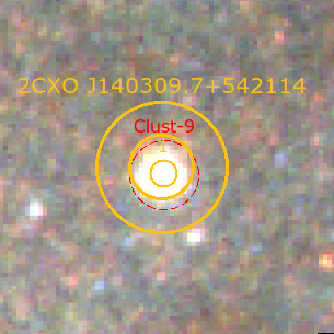
Fig. 11 Example of a standard globular cluster in M101. Notice, the globular cluster here is large enough to fill the 1-\(\sigma\) radius of this XRB and is much larger than the 3 pixel aperture plotted surrounding its centroid. This demonstrates why it is necessary to set a separate aperture radius for extended sources like star clusters, compared to isolated stars (e.g. the other, smaller point sources visible in the image).

To run RunPhots(), you will simply need to read in the FITS HDU, the galaxy name, the instrument (ACS/WFC or WFC3/UVIS), and the filter, though you pre-define additional parameters as well:

from XRBID.AutoPhots import RunPhots

# Running analysis on full mosaic. Can be done on individual
# fields using the 'suffix' parameter to differentiate savefile names
hdu = fits.open("M101_mosaic_acs_f555w_drc_sci.fits")

RunPhots(hdu, gal="M101", instrument="acs", filter="F555W", 
         fwhm_arcs=0.3, num_stars=25, reg_correction=[1,1], extended_rad=5)

Note

I choose to apply an additional pixel correction to the region files that result from RunPhots() by setting reg_correction = [1,1], which shifts all circular regions by 1 pixel in the x direction and 1 pixel in the y direction. This is because I noticed a small offset in the region files created from the coordinates of the point sources obtained by photutils aperture photometry. I don’t know what causes this disconnect, but since I intend to align the Chandra source coordinates to the HST region file coordinates, I use reg_correction to make sure the HST region file is properly aligned to the HST image.

This code may take a few minutes to run for each step, depending on the size of your FITS file. Then, it will prompt you to select ‘ideal’ stars for the aperture corrections by plotting the integrated radial profiles of randomly selected stars and requesting user approval.

The idea behind an aperture correction is to ensure that all of the light from a given star is captured and reflected in its measured flux/magnitude; since an aperture of infinite radius will detect the flux of an infinite number of sources other than the one you’re interested in, you need to select an aperture small enough to only measure the light from your selected star, but this aperture will undoubtedly ‘miss’ some of the light the star is giving off. An aperture correction is a means by which you can estimate and correct for the light that is presumably ‘cut off’ when you select an aperture of a given size. To do so, one should look at the radial profile of a given star and measure the flux/magnitude difference between the preferred aperture size (I use 3 pixels) and some larger aperture (e.g. 20 pixels). One then adds an additional correction factor measured from that larger aperture to infinity using the known Encircled Energy Fractions (EEF) for the instrument of choice[3]. Theoretically, this should estimate all of the light one expects to miss for an ideal star within a given HST observation, and this correction term can be applied to all remaining stars to get a better estimate of their total fluxes.

A good ‘ideal star’ is one with a magnitude that increases up until about 3 pixels, and then flattens off (see Fig. 12). RunPhots() will continue prompting the user for input until the number of ideal stars selected equals the input num_stars (the default is 20). As you add stars to the list of ideal stars, you will see their radial profiles plotted in grey, against which you can compare the radial profiles of the next randomly selected star. If you find that the same stars are being cycled through (as indicated by the star number in the title of the plot), this probably means there aren’t enough acceptable stars to meet the input criterion, and you should lower num_stars and try again. Once the criterion is met, RunPhots() will calculate and return the aperture correction and standard deviation. It may be a good idea to run the aperture correction a few times to make sure you’re minimizing the standard deviation, or you may not end up with an appropriate aperture correction. You can run just the aperture correction part of the code by calling AutoPhots.CorrectAp().

As of version 1.5.0, RunPhots() and CorrectAp() will also calculate the aperture correction for extended source given the aperture radius provided by the extended_rad parameter. By default, this value is 10 pixels, but one should select an aperture radius that best suits the compact clusters within the image of interest since farther galaxies will likely have clusters with smaller angular sizes. RunPhots() will then print *_extended.ecsv files from which the aperture photometry of clusters can be pulled.

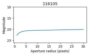
Fig. 12 The radial profile of an `ideal’ star, showing the total flux (converted to magnitudes) within an aperture of a given radius. The integrated flux of stars in HST images will generally max out by 3 pixels and should be flat at increasing radius. If there are wiggles/spikes in the flux, this suggests the star is non well-isolated (light from a nearby star is interfering with the measurement), and that star should not be used for the aperture correction.

Manual Source Identification and Photometry (w/o RunPhots())

For those who prefer to run their own point source identification, whether because RunPhots() did not produce acceptable results or because you value the skill, you can extract sources using photutils instead, which should already be included in your python installation. The following instructions walk you through one means of manually identifying point sources in your HST images, extracting their photometry, and estimating an aperture correction for each image/filter, which you can use instead of RunPhots(). There almost certainly are other methods that you could use as well, but those will not be discussed here.

Identifying Point Sources with DAOStarFinder

The main function used to find stars in a FITS file is the DAOStarFinder[4] function. This requires an estimate of the FWHM of stars on the image and some threshold amplitude above which a detection is found.

Open the FITS file in your imaging software of choice and use the analytics of that software to determine some reasonable measurement of the background noise in a dark area of the image, and the FWHM of a few average stars. For DS9, you can use the instructions in Using AutoPhots.RunPhots() for Everything to find the FWHM. An important thing to note is that DAOStarFinder requires the FWHM in pixels, but DS9 gives it in arcseconds. The pixel scale for is 0.05 arcsec per pixel for ACS/WFC and 0.03962 for WFC3/UVIS. This is usually stored under the FITS HDU header D001SCAL.

The background noise measurement is used to estimate a good threshold above which DAOStarFinder should search for stars. I use the standard deviation of the flux, which can be found easily in CARTA using the ‘Statistic Widget’ (the calculator button) on a selected region. This can also be obtained in python using sigma_clipped_stats from astropy.stats. I then use this value to define the threshold (by default, I use a threshold of 5 times the standard deviation):

from astropy.io import fits
from astropy.stats import sigma_clipped_stats
from photutils.detection import DAOStarFinder

fwhm = 0.3        # in arcseconds, from DS9
pixtoarcs = 0.05  # arcsec/pix, for ACS/WFC
data = fits.getdata('M101_mosaic_acs_f555w_drc_sci.fits')

# You can define some other sigma, depending on the quality of your data
dat_mean, dat_med, dat_std = sigma_clipped_stats(data, sigma=5)

# Pulling sources using DAOStarFind
daofind = DAOStarFind(fwhm=fwhm/pixtoarcs, threshold=5*dat_std)
objects = daofind(data)

DAOStarFind will return a table containing the coordinates of all identified sources, which can be used to make a region file that will plot in DS9 and CARTA (this can be done easily using my custom function WriteScript.WriteReg()). For reasons I don’t understand, the region file that comes from these coordinates often doesn’t align very well with the image itself, even though I believe the photometry that comes from these coordinates is accurate. When creating a region file, it may be a good idea to do a minor coordinate shift, just so that the regions align with the image and don’t cause confusion during the aperture correction step. Also, you’ll want to check the region file to make sure DAOStarFind isn’t missing any obvious sources. If it is, you’ll need to adjust your parameters (such as the FWHM) and run it again.

Extracting Photometry with aperture_photometry

RunPhots() will conduct the aperture photometry for you with a default minimum radius of 3 pixels, but you can also run the aperture photometry yourself with photutils.aperture_photometry. The inputs for aperture_photometry are fairly simple: all you need is the FITS data (background subtracted) and a list of aperture radii at the positions of your sources of interest, built with photutils.aperture.CircularAperture(). Using the resulting objects table obtained from DAOStarFinder above:

from photutils.aperture import CircularAperture

# Pulling position of each DAOStarFind source
positions = np.transpose((objects['xcentroid'], objects['ycentroid']))

# Taking aperture photometry on a range of apertures from 1-30 pix
ap_rads = [i for i in range(1,31)]
apertures_full = [CircularAperture(positions, r=r) for r in ap_rads]

There are probably a couple of ways to generate a background subtracted image from the FITS data, but the way I prefer uses tools from photutils.background combined with SigmaClip from astropy.stats:

from photutils.background import Background2D, MedianBackground
from astropy.stats import SigmaClip

sigma_clip = SigmaClip(sigma=5)
bkg_estimator = MedianBackground()
bkg = Background2D(data, (50, 50), filter_size=(3, 3), 
                   sigma_clip=sigma_clip,
                   bkg_estimator=bkg_estimator)
data_sub = data - bkg.background

This background-subtracted data can then be used in the aperture photometry extraction (for cleaner photometry, you can also add an error calculation):

from photutils.aperture import aperture_photometry

phot_full = aperture_photometry(data_sub, apertures_full, method="center")

# or, alternatively, to include an error calculation
from photutils.utils import calc_total_error

hdu = fits.open('M101_mosaic_acs_f555w_drc_sci.fits')
phot_full = aperture_photometry(data_sub, apertures_full, 
    		            error=calc_total_error(data, data-data_sub,
    				  effective_gain=hdu[0].header["EXPTIME"]))

phot_full.write("<filename>.ecsv")

The resulting .ecsv file will contain the coordinates of each source and the integrated flux within each aperture radius (in this case, 1–30 pixels). For normal stars, I generally use the flux within a 3-pixel aperture to represent a single star, as this radius is usually large enough to collect most of the stellar light but small enough for the flux not to be influenced by contamination from a neighboring star. However, any defined aperture is sure to miss some of the light of the chosen star, which is why an aperture correction is also needed to fully represent the stellar flux of a star of interest.

Estimating Aperture Corrections

RunPhots() will automatically conduct the aperture corrections using a second custom function, CorrectAp(). The philosophy behind aperture corrections is described in detailed above in Using AutoPhots.RunPhots() for Everything or, in a more official capacity, here: https://www.stsci.edu/hst/instrumentation/acs/data-analysis/aperture-corrections

To perform a manual aperture correction, you will want to select a sufficient number of ‘ideal’ isolated stars and find the magnitude difference between the 3 pixel and 20 pixel aperture photometry for each star[5]. Plot their radial profiles to check that it looks similar to the ideal case represented by Fig. 12. The median of these difference values (or some other well-argued statistical measure) is the correction term you will apply to the 3-pixel photometry of all other stars of interest. An additional term representing the magnitude difference between the 20 pixel radius and infinity should also be applied; this value can be found in the aperture correction link above for ACS/WFC, or here for WFC3/UVIS: https://www.stsci.edu/hst/instrumentation/wfc3/data-analysis/photometric-calibration/uvis-encircled-energy

This EEF value is given as the fraction of the light encircled by the maximum aperture, which should be used to calculate how much more light needs to be added to capture 100% of the stellar emissions (that is, out to infinity).

Be sure to save these values for each filter, as well as their standard deviations. For my data, I obtained the following values:

ap555_acs = -0.711
ap555err_acs = 0.220
ap435_acs = -0.660
ap435err_acs = 0.248
ap814_acs = -0.561
ap814err_acs = 0.253

The values are negative because they are to be added to the magnitudes from the 3-pixel aperture photometry representing a given star. More negative magnitudes indicate brighter stars, and the aperture correction should make the star appear brighter as we add back the missing light.

---

[1]

The procedure previously used by [ChandarJohnsMok+20] used the IRAF package called DaoPhots, found here: https://www.star.bris.ac.uk/~mbt/daophot/ . While you can certainly do this, I prefer to use the python equivalent, which I find is more flexible and a bit easier to work with.

[2]

You can probably use CARTA to measure FWHM as well, but I haven’t tested this.

[3]

For more information, see https://www.stsci.edu/hst/instrumentation/acs/data-analysis/aperture-corrections (for ACS/WFC) or https://www.stsci.edu/hst/instrumentation/wfc3/data-analysis/photometric-calibration/uvis-encircled-energy (for WFC3/UVIS)

[4]

https://photutils.readthedocs.io/en/2.0.2/api/photutils.detection.DAOStarFinder.html

[5]

3 and 20 pixels are the typical apertures I use to represent a star and its environment, respectively. However, you may choose to use a different minimum and maximum radius, so long as the minimum radius sufficiently isolates your chosen star from the flux of its environment, and the maximum radius is sufficiently far from the star to capture that plateau of the stellar flux as the light fades into the background. You will want your choice in maximum radius to be one that is found in the EEF tables for the observing instrument, or at least close to one of radii given.