
Retrieving X-ray Data from the CSC#
For my work, the most important information that I need from CXO is the coordinates of the X-ray sources (used to locate their optical counterparts on an HST image), their X-ray luminosities (calculated from the CSC-provided flux), their hardness ratios (used to determine whether or not they may be a supernova remnant in a later section), the off-axis angle, and the total X-ray counts (the last two of which are used to calculate the uncertainty radii in Astrometric Corrections). This information can be pulled directly from CSCView.jar.
Open the program by clicking the icon or typing into the command line (where it is saved):
java -jar cscview.jar &
(The optional & allows you to continue using the terminal for other processes while cscview.jar is running)
This will open the program GUI, which will look something like:
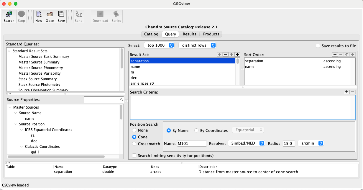
Select the most recent data release and press the Search button at the top left to be brought from the Catalog tab to the Query tab.
In the Query tab under Source Properties, search for hardness ratio (hard_hs) and add it to the Result Set with the + button. Do the same for off-axis angle (theta or theta_mean) and total X-ray counts (I choose to use src_cnts_aper_b, src_cnts_aper_lolim_b, and src_cnts_aper_hilim_b, which appears to be what is used in [LehmerEufrasioTzanavaris+19]).
All other results can be left as is, or you may remove the properties that you won’t need to save memory. You can save the query settings for future use by clicking the Save button at the top of the window. By default, it is saved with the suffix .prop.
Note
There may be additional data needed in order to clean up the X-ray source catalog such that only good data are included in your analysis. Since I focused mainly on X-ray sources identified in [LehmerEufrasioTzanavaris+19], which did this step for me, I never had to deal with this. However, it’s something that will need to be kept in mind for future projects. See [LehmerEufrasioTzanavaris+19] for more information on data selection from CSC.
To search for the CXO X-ray sources associated with your galaxy of interest, select Cone under Position Search at the bottom of the window and search for the galaxy of interest by name or coordinates. In the example above, I am looking for X-ray sources in M101, which has a linear diameter of roughly 30 arcminutes. I set the search parameters accordingly and hit the Search button at the top left of the window. This automatically brings you from the Query tab to the Results tab, from which you can select all the X-ray sources and save them to a .vot file.
Important
You will need to press the Search button every time you make a change in the Query tab. Otherwise, your search results may not be updated!
To view the .vot file, open TopCat:
java -jar topcat-full.jar
(or whatever equivalent you saved it under). This will open a window that resembles the following:
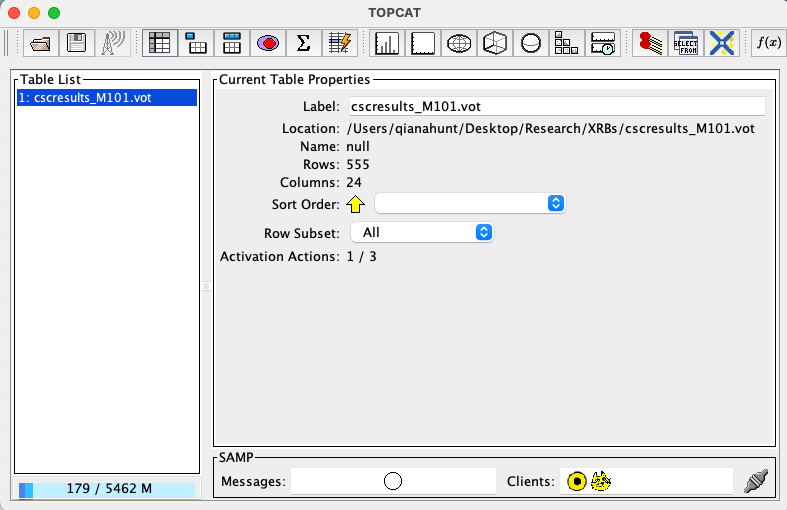
Fig. 1 Example of the TOPCAT user interface.#
In the GUI above, navigate to the .vot file via the Filestore Browser or System Browser interface. This will pull up the file information under Current Table Properties. The 4th icon at the top of the window (looks like a spreadsheet) will open the Table Browser, which allows you to view the table as a spreadsheet.
Converting from VOTable to Pandas DataFrame#
The XRBID package contains a specialized function for converting .vot files from the CSC into Pandas DataFrames in python: XRBID.Sources.NewSources(). To use this function, you simply need to run something like this in python:
from XRBID.Sources import NewSources

# Note: I saved my .vot to a directory called 'testdata',
#       so that's included in my filename path below
TempSources = NewSources("../testdata/cscresults_M101.vot")
display(TempSources)
Reading in table from ../testdata/cscresults_M101.vot
DONE
| separation | name | ra | dec | livetime | theta_mean | err_ellipse_r0 | err_ellipse_r1 | err_ellipse_ang | significance | ... | hard_hs_hilim | hard_hm | hard_hm_lolim | hard_hm_hilim | hard_ms | hard_ms_lolim | hard_ms_hilim | src_cnts_aper_b | src_cnts_aper_lolim_b | src_cnts_aper_hilim_b | |
|---|---|---|---|---|---|---|---|---|---|---|---|---|---|---|---|---|---|---|---|---|---|
| 0 | 0.835778 | 2CXO J140312.5+542056 | 210.802227 | 54.348952 | 192658.710333 | 2.687974 | 0.296164 | 0.295254 | 89.606978 | 22.302136 | ... | -0.454091 | 0.028732 | -0.100562 | 0.156777 | -0.553404 | -0.61649 | -0.485322 | 170.006026 | 155.698239 | 184.313814 |
| 1 | 0.835778 | 2CXO J140312.5+542056 | 210.802227 | 54.348952 | 142729.493705 | 2.727056 | 0.296164 | 0.295254 | 89.606978 | 22.302136 | ... | -0.454091 | 0.028732 | -0.100562 | 0.156777 | -0.553404 | -0.61649 | -0.485322 | 254.489381 | 233.532285 | 274.136658 |
| 2 | 0.835778 | 2CXO J140312.5+542056 | 210.802227 | 54.348952 | 141298.623812 | 2.783596 | 0.296164 | 0.295254 | 89.606978 | 22.302136 | ... | -0.454091 | 0.028732 | -0.100562 | 0.156777 | -0.553404 | -0.61649 | -0.485322 | 442.576953 | 419.112035 | 464.477543 |
| 3 | 0.835778 | 2CXO J140312.5+542056 | 210.802227 | 54.348952 | 132129.439441 | 2.690653 | 0.296164 | 0.295254 | 89.606978 | 22.302136 | ... | -0.454091 | 0.028732 | -0.100562 | 0.156777 | -0.553404 | -0.61649 | -0.485322 | 131.798703 | 118.539780 | 144.321019 |
| 4 | 0.835778 | 2CXO J140312.5+542056 | 210.802227 | 54.348952 | 130186.649966 | 2.749161 | 0.296164 | 0.295254 | 89.606978 | 22.302136 | ... | -0.454091 | 0.028732 | -0.100562 | 0.156777 | -0.553404 | -0.61649 | -0.485322 | 649.590529 | 616.129127 | 683.051932 |
| ... | ... | ... | ... | ... | ... | ... | ... | ... | ... | ... | ... | ... | ... | ... | ... | ... | ... | ... | ... | ... | ... |
| 3487 | 892.520732 | 2CXO J140447.2+542633 | 211.196627 | 54.442543 | 120993.038017 | NaN | 1.612100 | 0.795238 | 86.007749 | 2.650000 | ... | NaN | NaN | NaN | NaN | NaN | NaN | NaN | 0.000000 | 0.000000 | 59.364933 |
| 3488 | 892.520732 | 2CXO J140447.2+542633 | 211.196627 | 54.442543 | 88598.047743 | NaN | 1.612100 | 0.795238 | 86.007749 | 2.650000 | ... | NaN | NaN | NaN | NaN | NaN | NaN | NaN | 0.000000 | 0.000000 | 14.952548 |
| 3489 | 892.520732 | 2CXO J140447.2+542633 | 211.196627 | 54.442543 | 81021.851289 | 13.486809 | 1.612100 | 0.795238 | 86.007749 | 2.650000 | ... | NaN | NaN | NaN | NaN | NaN | NaN | NaN | 53.481053 | 29.414579 | 77.547526 |
| 3490 | 892.520732 | 2CXO J140447.2+542633 | 211.196627 | 54.442543 | 52087.100775 | NaN | 1.612100 | 0.795238 | 86.007749 | 2.650000 | ... | NaN | NaN | NaN | NaN | NaN | NaN | NaN | 0.000000 | 0.000000 | 34.780341 |
| 3491 | 892.520732 | 2CXO J140447.2+542633 | 211.196627 | 54.442543 | 14276.493764 | 3.416463 | 1.612100 | 0.795238 | 86.007749 | 2.650000 | ... | NaN | NaN | NaN | NaN | NaN | NaN | NaN | 7.591890 | 4.313574 | 10.870206 |
3492 rows × 28 columns
Keep in mind, the code will need to point towards where your .vot file(s) are saved on your computer! If you would like to save this to a file, you can do so in one of two ways: either save it using functions native to Pandas, or use the outfile parameter in NewSources():
# Saving the file using Pandas
TempSources.to_csv("../testdata/cscresults_M101.frame") # Pandas version of saving the df

# Alternatively, saving file using NewSources
TempSources = NewSources(infile="../testdata/cscresults_M101.vot",
                         outfile="../testdata/cscresults_M101.frame")
Reading in table from ../testdata/cscresults_M101.vot
Reading in sources from ../testdata/cscresults_M101.frame...
DONE
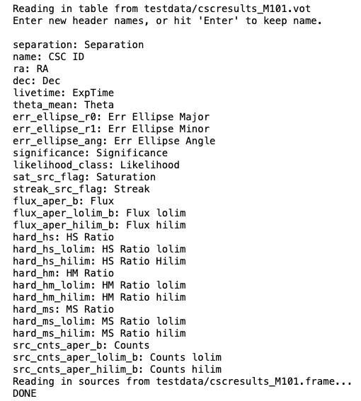
As you can see, the calls to NewSources above will read in the table exactly as written. If you want to rename the headers, you can do so manually in the .frame file created above or by setting the rename parameter to True. The code below will prompt you to rename each of the headers within the .vot table, then save the DataFrame as a comma-separated value (CSV):
NewSources(infile="../testdata/cscresults_M101.vot", rename=True,
           outfile="../testdata/cscresults_M101_renamed.frame")
The CSV output file created above (cscresults_M101.frame) is easily read in by pd.read_csv() or XRBID.Sources.LoadSources(). The latter is a little slower, but it will automatically remove the index column of the CSV file and convert applicable values from strings into actual numbers as the DataFrame is being built. This is usually very helpful during the analysis stage, so I recommend using LoadSources() when you can.
You should also save these sources as a region file that can be loaded into DS9 or CARTA to overlay onto an HST FITS file. This can be done fairly simply with XRBID.WriteScript.WriteReg() – for example:
from XRBID.WriteScript import WriteReg
from XRBID.Sources import LoadSources

TempSources = LoadSources("../testdata/cscresults_M101_renamed.frame")
display(TempSources)

# Writing to a DS9-compatible region file
WriteReg(TempSources, outfile="../testdata/cscsources_M101.reg", idname="CSC ID",
        radius=50, width=2, color="hotpink", showlabel=True)
Reading in sources from ../testdata/cscresults_M101_renamed.frame...
| Separation | CSC ID | RA | Dec | ExpTime | Theta | Err Ellipse Major | Err Ellipse Minor | Err Ellipse Angle | Significance | ... | HS Ratio hilim | HM Ratio | HM Ratio lolim | HM Ratio hilim | MS Ratio | MS Ratio lolim | MS Ratio hilim | Counts | Counts lolim | Counts hilim | |
|---|---|---|---|---|---|---|---|---|---|---|---|---|---|---|---|---|---|---|---|---|---|
| 0 | 0.835778 | 2CXO J140312.5+542056 | 210.802227 | 54.348952 | 192658.710333 | 2.687974 | 0.296164 | 0.295254 | 89.606978 | 22.302136 | ... | -0.454091 | 0.028732 | -0.100562 | 0.156777 | -0.553404 | -0.61649 | -0.485322 | 170.006026 | 155.698239 | 184.313814 |
| 1 | 0.835778 | 2CXO J140312.5+542056 | 210.802227 | 54.348952 | 142729.493705 | 2.727056 | 0.296164 | 0.295254 | 89.606978 | 22.302136 | ... | -0.454091 | 0.028732 | -0.100562 | 0.156777 | -0.553404 | -0.61649 | -0.485322 | 254.489381 | 233.532285 | 274.136658 |
| 2 | 0.835778 | 2CXO J140312.5+542056 | 210.802227 | 54.348952 | 141298.623812 | 2.783596 | 0.296164 | 0.295254 | 89.606978 | 22.302136 | ... | -0.454091 | 0.028732 | -0.100562 | 0.156777 | -0.553404 | -0.61649 | -0.485322 | 442.576953 | 419.112035 | 464.477543 |
| 3 | 0.835778 | 2CXO J140312.5+542056 | 210.802227 | 54.348952 | 132129.439441 | 2.690653 | 0.296164 | 0.295254 | 89.606978 | 22.302136 | ... | -0.454091 | 0.028732 | -0.100562 | 0.156777 | -0.553404 | -0.61649 | -0.485322 | 131.798703 | 118.539780 | 144.321019 |
| 4 | 0.835778 | 2CXO J140312.5+542056 | 210.802227 | 54.348952 | 130186.649966 | 2.749161 | 0.296164 | 0.295254 | 89.606978 | 22.302136 | ... | -0.454091 | 0.028732 | -0.100562 | 0.156777 | -0.553404 | -0.61649 | -0.485322 | 649.590529 | 616.129127 | 683.051932 |
| ... | ... | ... | ... | ... | ... | ... | ... | ... | ... | ... | ... | ... | ... | ... | ... | ... | ... | ... | ... | ... | ... |
| 3487 | 892.520732 | 2CXO J140447.2+542633 | 211.196627 | 54.442543 | 120993.038017 | NaN | 1.612100 | 0.795238 | 86.007749 | 2.650000 | ... | NaN | NaN | NaN | NaN | NaN | NaN | NaN | 0.000000 | 0.000000 | 59.364933 |
| 3488 | 892.520732 | 2CXO J140447.2+542633 | 211.196627 | 54.442543 | 88598.047743 | NaN | 1.612100 | 0.795238 | 86.007749 | 2.650000 | ... | NaN | NaN | NaN | NaN | NaN | NaN | NaN | 0.000000 | 0.000000 | 14.952548 |
| 3489 | 892.520732 | 2CXO J140447.2+542633 | 211.196627 | 54.442543 | 81021.851289 | 13.486809 | 1.612100 | 0.795238 | 86.007749 | 2.650000 | ... | NaN | NaN | NaN | NaN | NaN | NaN | NaN | 53.481053 | 29.414579 | 77.547526 |
| 3490 | 892.520732 | 2CXO J140447.2+542633 | 211.196627 | 54.442543 | 52087.100775 | NaN | 1.612100 | 0.795238 | 86.007749 | 2.650000 | ... | NaN | NaN | NaN | NaN | NaN | NaN | NaN | 0.000000 | 0.000000 | 34.780341 |
| 3491 | 892.520732 | 2CXO J140447.2+542633 | 211.196627 | 54.442543 | 14276.493764 | 3.416463 | 1.612100 | 0.795238 | 86.007749 | 2.650000 | ... | NaN | NaN | NaN | NaN | NaN | NaN | NaN | 7.591890 | 4.313574 | 10.870206 |
3492 rows × 28 columns
Saving ../testdata/cscsources_M101.reg
The code above takes every source in TempSources (i.e. every row in the DataFrame) and writes the coordinates to a DS9-compatible region file called cscsources_M101.reg. The default coordinate system here is galactic coordinates (or fk5 in DS9), since the DataFrame only contains RA and Dec coordinates. By setting showlabel = True and idname = "CSC ID", each circular region (representing the X-ray sources from CSC) will be labeled with the source ID taken from CSC and stored under the header “CSC ID”.
Note
For more information on additional parameters taken in by WriteReg(), one can run help(WriteReg) in python. This can be done with any python function.