Retrieving Optical Images from the HLA#
Note
If you intend to make a mosaic of your galaxy, this step can usually be skipped. It is recommended, however, that you look at what images are available in MAST or the HLA and jot down the PropID, Spectral_Elt, and Detector of images you want to use to make the mosaic step easier! See Creating Mosaics with AstroDrizzle
There are two ways to retrieve data from the HLA. The first is manually, and the second requires you to query the HLA from within python. The benefit to the latter technique is that this makes data retrieval practically automatic, although it does require a lot of user input that may take longer than it’s worth, depending on your workflow. It also allows you to pull data directly from from archive without having to download it to your computer, which is an enormous memory saver! However, with the way I’ve written my query, I’ve found it may not capture all HST images available on the HLA. I haven’t figured out how to solve for that issue quite yet. The only solution I have for now is to double-check everything with the manual process, and download any data that may be missing from the automatic query onto your computer to incorporate into your workflow.
First, I will demonstrate the manual way to retrieve HST data. Then, I will demonstrate the use of XRBID.ImageSearch for automatic data retrieval. Again, use the latter with caution, as it takes a long time and doesn’t always return all of the data available!
Manual Image Searches#
For projects in which many XRBs of a single galaxy are being surveyed, it’s recommended to do a manual image search (unless you’re making a mosaic, in which case you can skip ahead to Creating Mosaics with AstroDrizzle). Otherwise, using the ‘automatic’ method may be far more time-consuming than it’s worth.
There are two methods for manual image retrieval: using the Hubble Legacy Archive (HLA), or using the STScI Mikulski Archive for Space Telescopes (MAST). Each has its benefits, so it’s mostly a matter of taste. MAST will lay out the HST footprints on top of an image of the target galaxy, making it easy to see everything that’s available and how they fit together, but it includes so much information that the search can be quite slow for well-studied galaxies. The HLA, on the other hand, does not always give you a mosaic view of all of the observations, but is often extremely quick when it comes to data retrieval.
Downloading Images from the HLA#
To pull images from the HLA, go to the website and type in the name of your galaxy. If the galaxy has been observed with HST, a list of observations will appear under the Inventory tab. For my research, I require observations using the WFC3/UVIS[1] or ACS/WFC[2] detectors. I narrow down the observations by specifying the detector under the Detector tab (to my knowledge, this can only be done one at a time).
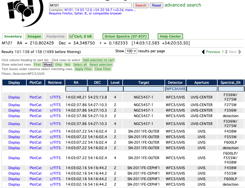
Fig. 2 Example search using the Hubble Legacy Archive.#
It’s useful to view what the actual images look like before downloading them. To do this, switch from the Inventory tab to the Images tab. Select the appropriate images (you’ll more than likely want the ones with science data) and add them to your cart by clicking the Download Data: FITS-Science link beneath each image. This will add them to the shopping cart tab, which you can use to retrieve your FITS data files once all desired images are selected.
Alternatively, you can click the More... link beneath each image to gather more information about the image (including the proposal ID needed for the AstroDrizzle step, which is the number beside ‘Information for HST observing program’) and to download the science data directly without adding it to the cart.
If you have files in your cart to download, you can do so by clicking on the Cart tab, selecting the Download Sequentially bubble (or Zipped File, if you prefer), and clicking Fetch HLA Data. This will initiate the download process. As these data files are usually pretty large, the download may take a while.
Downloading Images from MAST#
Alternatively, you can use the STSci MAST database to get a better visual of how much of the galaxy has been covered and by what filters. This is usually a good option, but be aware that the target search includes all observations made by all telescopes in the database, so if you are searching for a well-documented galaxy, it may take a very long time to load!
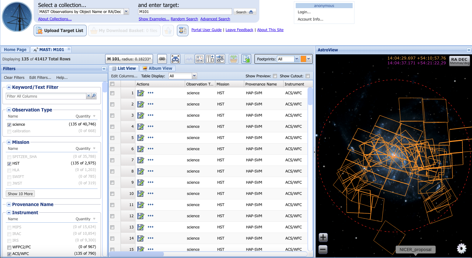
Fig. 3 Example search using the STSci MAST database. Here, the search was narrowed down to include only HST ACS/WFC science (HAP-SVM) observations made with the F435W, F555W, and F814W filters.#
To download data from MAST, narrow down the search results in the Filters tab on the left; in particular, you will want to select science in the Observation Type drop-down list, HST or HLA in Missions, ACS/WFC or WFC3/UVIS (or whatever other detectors you need for your specific project) in Instrument, and, if you want, the Filters of interest. You can then select the images you are interested in by either checking the appropriate box in the List View (center table) or clicking the footprint squares in the AstroView image on the right (see Fig. 3). You can also switch from List View to Album View to see exactly which images corresponds to which square in the AstroView section.
Add the images to your basket by clicking the button above the List View and Album View table that looks like an orange basket with 3 green arrows pointing into the basket (the button that is second from the end, greyed out, in Fig. 3). This will bring you to the Download Basket. Select the files you want to download and click the Download button on the top right. This will download the images in a series of nested directories, which you will likely want to reorganize in accordance with your preferred workflow.
If you intend to do a mosaic and do not want to run a search for images through astroquery (e.g. because your galaxy is nested within an proposed observation containing far more images than needed, etc.), then you can download the FLC files that you will need by deselecting the “Minimum Recommended Products” checkbox Download Manager window and selecting FLC from the Group filter.
Automatic Image Searches#
If your project requires images of only a couple of X-ray sources, or a handful of X-ray sources scattered across a sample of different galaxies, then you may find it useful to conduct a ‘automatic’ image search. It’s important to note that these searches aren’t fully automatic and require some input from the user, which is why they may not be ideal for studies of hundred of X-ray sources at a time. If you aren’t sure which search is best for your purposes, a manual search is usually sufficient, unless you are worried about storage space on your computer.
python HLA query with PyVO#
The code that I use for querying the HLA through python is included in XRBID.ImageSearch. This is heavily based on PyVO[3], which you should have already installed during the setup phase, and is mostly useful when you have a small number of sources to analyze.
To use ImageSearch.FindHST(), you will need to provide the function with either a list containing the RA and Dec of a single source (in units degrees), or a DataFrame containing the coordinates of multiple sources. So, for example, either :
FindHST([<RA>, <Dec>], galaxy = <galaxy>, savefile = <file>)
or
FindHST(<DataFrame>, galaxy = <galaxy>, savefile = <file>)
will work, as long as the coordinates, galaxy name, and some output file name are given. In either case, FindHST() will search the HLA for any optical image containing the coordinates given and present them as a list – first searching for ACS/WFC observations, then searching for WFC3/UVIS observations. Upon user request, it will plot the images with the coordinate of the source marked as a red X and prompt the user to input the indices of the best image files to save. You will want to select at least one image for each of the filters you’re interested in, where applicable. It will then save the image information to a .csv file matching your designated savefile name. This .csv will include a URL that can be used to read in the image file directly from the HLA without having to download the image to your computer!
If you just want to use FindHST() to look for all images associated with the galaxy, not necessarily for each individual XRB, you can do so by providing the coordinates of the galaxy and setting the search radius to the radius of the galaxy, in arcseconds. This will likely return many potential images, so in this case it’s recommended to save the initial HLA search using the savesearch parameter and decide in conjunction with the HLA website which images are appropriate from that image list. For example:
from XRBID.ImageSearch import FindHST

FindHST([210.802368, 54.359667], galaxy='M101', search_rad=900,
        savefile='Obslog_M101.csv', savesearch='M101_HLAsearch.csv')

# This code will produce a table with nearly 200 images.
# You can choose to go through each one sequentially,
# or use the M101_HLAsearch.csv + HLA to identify the best images manually
On the other hand, if you read in a DataFrame instead of a single pair of coordinates, then you will want to only use sources from a single galaxy at a time, and you’ll want to have a header containing some form of a source ID, which the code will prompt you to provide (for example, CSC ID). Currently, this code can only handle a single galaxy at a time, but this can be fairly easily updated to search for a galaxy header in the DataFrame in the future.
The downside of this procedure (as opposed to the manual HLA search) is that if you’re reading in a DataFrame containing all X-ray sources in a galaxy, then you will need to confirm the appropriate HST image for every XRB individually, which can take a lot of time for galaxies with many XRBs. However, you will not need to download the actual FITS files to access them, which saves a ton of memory and makes reading in each image faster. This procedure also saves all of the HST information about the observation that you could need, which is an added bonus that comes in handy when you’re writing a paper on your results!
python HLA query with astroquery#
As an alternative to PyVO, one can use astroquery to find and download HST data. PyVO is still a requirement for astroquery, so even if you decide not to use the PyVO method above, you’ll probably still need to install it. I use astroquery in Creating Mosaics with AstroDrizzle as part of my drizzling workflow, as it will find the FLC files needed for the drizzling and mosaic creation for you. For more information, see Downloading HST Observations with astroquery.
Handling HST Data#
The image data files from HST is given in FITS format[4]. This may be read in as an HDU[5] object with some form of python code resembling:
from astropy.io import fits
hdu = fits.open(<FITS file name>)
hdu.info()
The last line of that code will print a name and type of data stored in the HDU object, as well as the index you can use to access the data (No.). The PRIMARY element contains information regarding the image observation and reduction (e.g. the instrument configuration, calibrations applied, exposure time, etc.), and can be accessed with .header via hdu[0].header, where the index used is the index of the primary data, or hdu['PRIMARY'].header.
Importantly, the image from which the photometry is extracted is (usually) stored under SCI. The header information under SCI may also contain a lot of good information, including image statistics like the signal-to-noise (if the image reduction team was thorough in their record keeping), so it’s a good idea to take a look. Keep in mind, if you choose to create a mosaic and set build=False in AstroDrizzle (see sec:astrodriz), the science data will be stored under PRIMARY rather than under its own extension.
If you used the automatic HLA search method (FindHST()), then you can read in the FITS file associated with each source using ImageSearch.GetFITS(), which requires you provide the name of the file saved by FindHST(), the source of interest, the detector (in my case, ACS/WFC or WFC3/UVIS), and the filter (e.g. F814W, F555W, etc). GetFITS() reads in the image URL and returns an HDU object, so instead of the code above (which you would use if you saved a FITS directly to your computer), you can use something like:
from XRBID.ImageSearch import GetFITS

hdu = GetFITS(infile=<FindHST savefile name>, source_id=<source ID>,
              detector=<'ACS/WFC' or 'WFC3/UVIS'>, filter=<filter>)
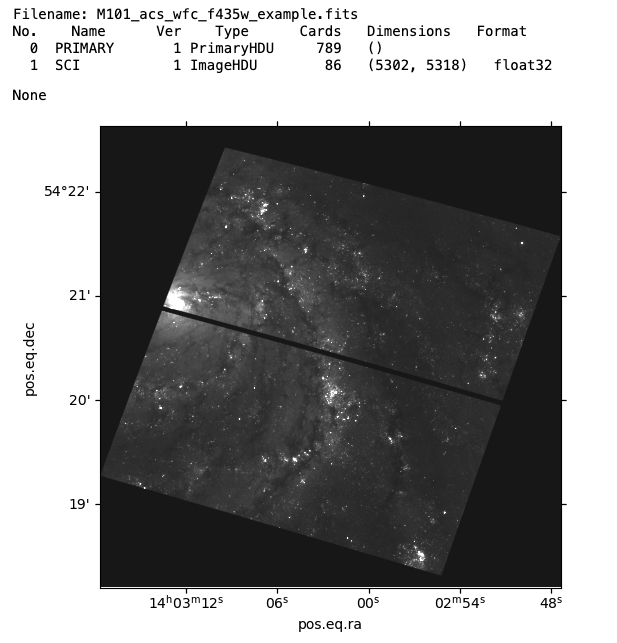
From the HDU object, a monochromatic image can be plotted using imshow() from matplotlib.pyplot. For these particular data, since light from a galaxy is logarithmic, you will also need to define a normalization parameter, norm. I tend to use matplotlib.colors.Normalize() with some specified vmin and vmax to change the scaling until the image looks right. For example:
import matplotlib
import matplotlib.pyplot as plt
from astropy.wcs import WCS # defining the coordinate system, e.g. RA/Dec
from astropy.io import fits

hdu = fits.open('../testdata/M101_acs_wfc_f435w_example.fits')
display(hdu.info()) # Display the hdu info to get more information about what it contains

# Setting up the figure
plt.figure(figsize=(6,6))

# hdu['SCI'].header usually contains info needed to set up the image projection
# But you may need to check your specific hdu file
ax = plt.subplot(projection=WCS(hdu['SCI',1].header))
plt.imshow(hdu['SCI',1].data, cmap="gray", origin="lower",
           norm=matplotlib.colors.Normalize(vmin=-0.05, vmax=.5))
plt.show()
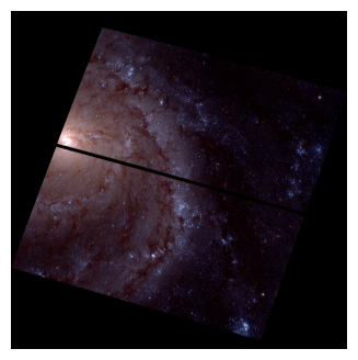
Plotting color images in python#
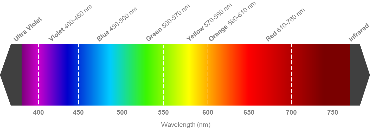
Whether you choose to plot color images in an imaging software like DS9 or in python, you will need at least three filters to get a full color image. The filters are then assigned to the red, green, or blue channels of DS9 or whatever python imaging code you use, based on the filter of each image. Below is an example of the visual electromagnetic spectrum; assign each filter image you have from HST based on which wavelength is closest to red, green, and blue on the visual spectrum.
To get a color image, you can use make_lupton_rgb() from astropy.visualization to generate a scaleable RGB color image, create your own logarithmic scaling algorithm, or simply use either
ImageSearch.MakePostage() or ImageSearch.PlotField() (which does basically the same, but is a semi-automatic plotting function that will lead you through each of the steps). Below is an example of creating a color image using a custom logarithmic scaling algorithm, which is my preferred method:
import numpy as np
from reproject import reproject_interp    # May need to install first

# Calling FITS files as the RGB filters
hdu_r = fits.open('../testdata/M101_acs_wfc_f814w_example.fits')
hdu_g = fits.open('../testdata/M101_acs_wfc_f555w_example.fits')
hdu_b = fits.open('../testdata/M101_acs_wfc_f435w_example.fits')
data_g = hdu_g['SCI'].data   # Pulling data from FITS HDU

# Resizing images that don't match the base HDU, hdu_g (required)
if hdu_r['SCI'].data.shape != hdu_g['SCI'].data.shape:
  data_r, _ = reproject_interp(hdu_r['SCI'], hdu_g['SCI'].header)
else: data_r = hdu_r['SCI'].data
if hdu_b['SCI'].data.shape != hdu_g['SCI'].data.shape:
  data_b, _ = reproject_interp(hdu_b['SCI'], hdu_g['SCI'].header)
else: data_b = hdu_b['SCI'].data

# Defining the min and max brightness cutoff of RGB image, per filter
# These are obtained through trial and error.
clipmin_r = 0.2
clipmax_r = 3.0
clipmin_g = 0.1
clipmax_g = 2.0
clipmin_b = 0.05
clipmax_b = 1.0

# Applying mag clipping and converting data to log
r = np.log10(np.clip(data_r, clipmin_r, clipmax_r))
g = np.log10(np.clip(data_g, clipmin_g, clipmax_g))
b = np.log10(np.clip(data_b, clipmin_b, clipmax_b))

# Rescaling the filters based on their individual min and max values
r_scaled = (r-np.nanmin(r))/(np.nanmax(r)-np.nanmin(r))
g_scaled = (g-np.nanmin(g))/(np.nanmax(g)-np.nanmin(g))
b_scaled = (b-np.nanmin(b))/(np.nanmax(b)-np.nanmin(b))
rgb_scaled = np.dstack((r_scaled,g_scaled,b_scaled))

# Plotting RGB image
plt.figure(figsize=(4,4))
ax = plt.subplot(projection=WCS(hdu_g['PRIMARY'].header))
plt.imshow(rgb_scaled)
plt.axis("off")
plt.show()